Machine Learning Ex2 - Linear Regression

Implementing linear regression using gradient descent in Scala based on Andrew Ng's machine learning course.


Stanford Univeristy recently announced that they will be offering thirteen online courses as part of their Stanford Engineering Everywhere program. According to the NYTimes, 58K people signed up for the Articial Intelligence course alone. Three days later, the number of interested students for that course went up to 100K.

Another course with much interest is Machine Learning, taught by professor Andrew Ng. There already exists a version of this course online, which is more of a series of video lectures and less of a classroom environment that has handouts and quizzes.

The original solution by professor Ng is done using MATLAB, the popular numerical programming language. Alexandre Martins decided to implement all the exercises of the course using R in his excellent blog. In the same spirit, I will use Scala instead. Scala's use of functional programming techniques and speed (thanks to the JVM) make it an ideal language for number cruching on large data sets.

THEORY

The linear regression model is a basic line that best fits the existing data points from the training set.
$$h_\theta(x) = \theta_0 x_0 + \theta_1 x_1 + \theta_2 x_2 + ...$$
The learned hypothesis in this example will be able to predict the height (y values) of a boy given their age (x values).

Batch gradient descent will basically attempt to minimize the cost function, which fits parameters of the model, by finding the values of theta that have the least square errors between the training set and the estimated values. The cost function for our linear model is defined as:
$$J(\theta) = \frac{1}{2m} \sum_{i=1}^m (h_\theta(x^{(i)}) - y^{(i)})^2$$
We will apply gradient descent by using the partial derivative of the cost function over x multiplied by a learning rate (alpha) to update theta. The process is repeated until we have reached convergence.
$$\theta_j := \theta_j - \alpha \frac{1}{m} \sum_{i=1}^m (h_\theta(x^{(i)}) - y^{(i)}) x^{(i)}$$

The preceding formula can be converted to linear algebra using basic matrix/vector operations.
$$\theta := \theta - \alpha \frac{1}{m} x^T (x\theta^T - y)$$

CODE

The first approach will be an iterative solution without using linear algebra. We will assume that for all values of x $$x_0 = 1$$

Note: the following code is meant to be run simply as a script inside the Scala REPL and not as part of some larger class-based solution.

 val x = io.Source.fromFile("ex2x.dat").getLines.toList map { x => List(1.0, x.toDouble) }  
 val y = io.Source.fromFile("ex2y.dat").getLines.toList map { y => y.toDouble }  
   
 val m = x.size  
 val alpha = 0.07  
   
 var theta = List(0.0, 0.0)  
   
 //  linear regression model
 val h: List[Double] => Double = { x => theta(0)*x(0) + theta(1)*x(1) }  
   
 // sum the difference (error) for each xy pair   
 // using the current values of theta  
 val delta: Int => Double = { idx =>  
  0 to m-1 map { i =>   
   val xi = x(i)  
   val yi = y(i)  
   (h(xi) - yi) * x(i)(idx)  
  } reduceLeft(_+_)  
 }  
   
 for (k <- 1 to 1500) {   
  // calculate theta values separately  
  val theta0 = theta(0) - (alpha * 1/m * delta(0))  
  val theta1 = theta(1) - (alpha * 1/m * delta(1))  
  theta = List(theta0, theta1)  
 }  

Result

 scala> theta  
 res: List[Double] = List(0.7501503917693573, 0.06388337549971077)  

Besides coming up with the algorithm for batch gradient descent, part of the exercise was to predict the height for two boys of age 3.5 and age 7. Using the values of theta, we can predict the values:

 scala> theta(0) + theta(1)*3.5  
 res: Double = 0.9737422060183449  
   
 scala> theta(0) + theta(1)*7  
 res: Double = 1.1973340202673326  

While the solution is not long, it leaves a lot to be desired. In the course, it is stated that a solution using linear algebra will often be simpler and more efficient if the right linear algebra library is used. For Scala, Scalala is a great linear algebra library that is developed as part of the ScalaNLP project. There are several existing Java linear algebra libraries, but Scala-specific libraries tend to be optimized with Scala goodies such as implicit conversions that make coding easier.

Easiest way to start using Scalala is to create a simple sbt project and define the following dependencies:

 val scalaToolsSnapshots = "Scala Tools Snapshots" at "http://scala-tools.org/repo-snapshots/"  
 val scalaNLPRepo = "ScalaNLP Maven2" at "http://repo.scalanlp.org/repo"   
 val OndexRepo = "ondex" at "http://ondex.rothamsted.bbsrc.ac.uk/nexus/content/groups/public"   
   
 val scalala = "org.scalala" %% "scalala" % "1.0.0.RC2-SNAPSHOT"  

The dependencies for the project can be downloaded with the update action in sbt, after which you can then proceed to use sbt's project console to start a Scala REPL with all library dependencies defined in the classpath.

Scalala expects the input values to be in a different format than the iterative version, so the first thing to do is create a matrix and vector for our x and y values. Once again, the x values have 1.0 in the first column since x0 is defined as 1 in our linear model.

 import scalala.tensor.dense._  
   
 val tempx = io.Source.fromFile("ex2x.dat").getLines.toList map { x => (1.0, x.toDouble) }  
 val tempy = io.Source.fromFile("ex2y.dat").getLines.toList map { y => y.toDouble }  
 val x = DenseMatrix(tempx:_*)  
 val y = DenseVector(tempy:_*)  
   
 val m = x.numRows // slight change  
 val alpha = 0.07  

With the setup out of the way, we can now find the values for theta using linear algebra.

 var theta = DenseVector(0.0, 0.0)  
   
 1 to 1500 foreach { _ =>   
  val grad = x.t * ((x * theta) - y) / m  
  theta = theta - (grad * alpha)   
 }  

Result

 scala> theta  
 res: scalala.tensor.dense.DenseVectorCol[Double] =   
  0.750150  
  0.0638834  

As theorized, the linear algebra solution was indeed much simpler. Two separate functions were reduced to a single line of code and there was no need to calculate the two values of theta independently.

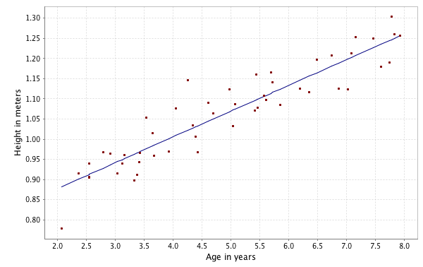
Scalala also provides a wrapper to the JFreeChart library for creating graphics. First let us plot the values from the training set:

 import scalala.library.Plotting._  
 import scalala.tensor.::  
   
 plot.hold = true // do not create a new figure for every plot call
 plot(x(::,1), y, '.')  

We can now plot a line of the linear fit

 plot(x(::,1), x*theta)  

Using linear algebra, we can also once again predict the height for the two boys:

 scala> DenseVector(1, 3.5).t * theta  
 res: Double = 0.9737422060183449  
   
 scala> DenseVector(1, 7).t * theta  
 res: Double = 1.1973340202673326  

UPDATE: all solutions benchmarked http://blog.brusic.com/2011/08/machine-learning-ex2-benchmarks.html